1.0 Introduction
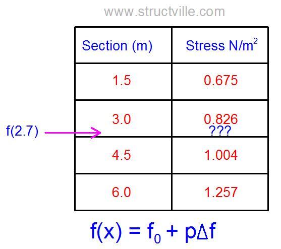
In the design of structures, engineers are always faced with the task of carrying out interpolations as supported by various codes of practice. These interpolations are often encountered when we are carrying out wind load analysis, designing our columns, designing our two-way slabs, etc.
Some people may not be very familiar with the process of linear interpolation, and this is the problem this post attempts to address, showing how to use Gregory-Newton forward difference formular for carrying out interpolations. I am not going to go through the process of deriving the formular, but I will present it exactly the way it is applied, and use practical examples to consolidate it.
2.0 Gregory-Newton Forward Difference Formular
Let x0, x1, x2,…, xn be equally spaced values, so that xi = x0 + ih, for i = 1, 2,…, n.
If the values f0, f1, f2,…, fn are known, where fi = f(xi), for some function f.
The Gregory–Newton forward difference formula is a formula involving finite differences that gives an approximation for f(x), where x = x0 + ph, and f(x) ≈ f0 + pΔf0 gives the result of linear interpolation. For each pair of consecutive function values f(x0) and f(x1), the forward difference is obtained by subtracting f(x0) from f(x1). However, when the series is terminated after one more term provides an example of quadratic interpolation.
In this post, we are considering linear interpolation only, and cases where it can be applied.
Quickly, let us use the table below to show how this process is carried out. The relationship between the values is fairly linear.
For the table given below, we are required to calculate the value of f(3.5).
Note that the value we seek (3.5) is between 3 and 4
So;
x0 = 3; x1 = 4; xp = 3.5
h = x1 – x0 = 4 – 3 = 1
p = (xp – x0)/h = (3.5 – 3)/1.0 = 0.5
Δf0 = f(x1) – f(x0) = 59 – 47 = 12
Therefore; f(3.5) = 47 + 0.5(12) = 53
This one is just as simple as that.
Now let us go into practical scenarios encountered in structural design.
3.0 Applications in Structural Design
Example 1
Calculation of bending moment coefficient for two-way slabs
Table 3.14 of BS 8110-1:1997 gives coefficients that are used to obtain the bending moment coefficients of rectangular slabs subjected to uniform pressure under various support conditions. This same coefficient is also used in the Eurocodes, and an excerpt is given below.
Let us assume that we have a slab with one short edge discontinuous with an aspect ratio of 1.46. We wish to obtain the positive bending moment coefficient for the mid-span by using linear interpolation.
x0 = 1.4; x1 = 1.5; xp = 1.46
h = x1 – x0 = 1.5 – 1.4 = 0.1
p = (xp – x0)/h = (1.46 – 1.4)/0.1 = 0.6
Δf0 = f(x1) – f(x0) = 0.043 – 0.041 = 0.002
Therefore; f(1.46) = 0.041 + 0.6(0.002) = 0.0422
I guess that was very simple and straightforward.
Example 2
External Wind Pressure coefficient on Buildings
Table 7.1 of EN 1991-1-4:2004 gives the recommended values of external pressure coefficients for buildings that are rectangular in plan. Design engineers usually encounter this table when carrying out wind load analysis. The code permits us to determine intermediate values by interpolation.
Let us assume that we are to determine Cpe,10 for a building in zone A, having a h/d ratio of 2.3
x0 = 1; x1 = 5; xp = 2.3
h = x1 – x0 = 5 – 1 = 4
p = (xp – x0)/h = (2.3 – 1)/4 = 0.325
Δf0 = f(x1) – f(x0) = -1.2 – (-1.2) = 0
Therefore; f(2.3) = -1.2 + 0.325(0) = -1.2
Example 3
Compressive Strength of Steel to BS 5950-1:2000
The slenderness ratio of a steel stanchion is 17.5, the grade of the steel is S275, and the thickness of the section is less than 40mm. So we are to interpolate from the table above to obtain the compressive strength.
x0 = 15; x1 = 20; xp = 17.5
h = x1 – x0 = 20 – 15 = 5
p = (xp – x0)/h = (17.5 – 15)/5 = 0.5
Δf0 = f(x1) – f(x0) = 271 – 275 = -4
Therefore; f(2.3) = 275 + 0.5(-4) = 273 N/mm2
Thank you for visiting Structville today. Your presence means so much to us.


Thank you , a nice piece indeed.