Finite element analysis has become an indispensable tool in structural engineering, enabling complex simulations of real-world scenarios through numerical methods. By discretizing a continuous structure into smaller finite elements, the governing equations describing its behaviour are transformed into a solvable system of algebraic equations.
The human mind, despite its remarkable capabilities, faces inherent limitations in comprehending the intricacies of complex systems in one single step. In response to this challenge, a fundamental approach emerges: decomposition or discretization of complex problems. By systematically dividing systems into their constituent elements whose behaviour is easily understood, we can then reconstruct the whole system to evaluate its overall response. This principle, employed by engineers, scientists, and even economists, forms the cornerstone of the finite element method.
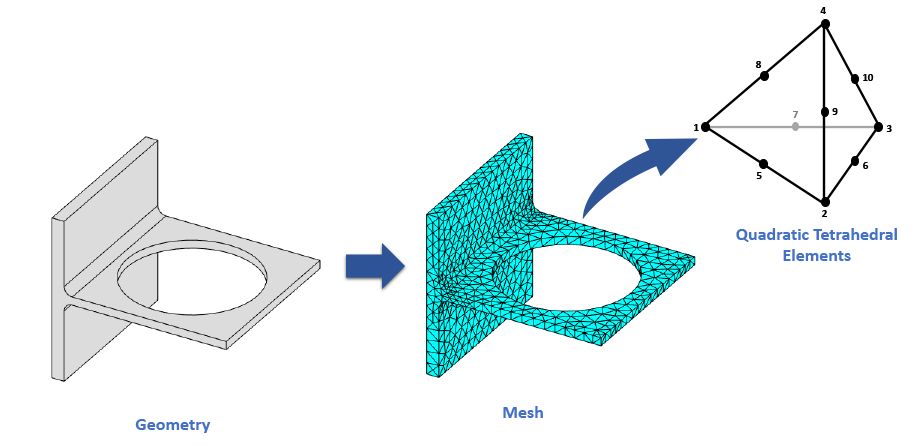
At its core, the finite element method seeks to approximate solutions to complex problems by substituting them with simpler counterparts. This inherent simplification necessitates an approximate, rather than exact, solution. The method achieves this by discretizing the solution domain into smaller, interconnected subregions – the finite elements. Depending on the system, a finite number of such elements can often sufficiently represent the true system, which we classify as discrete.
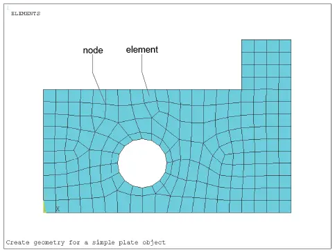
However, certain systems require infinite subdivision, demanding the mathematical abstraction of infinitesimals. This leads to differential equations or their equivalent, implying an infinite number of elements, characterizing continuous systems. While digital computers excel at solving large-scale discrete problems, their finite capacity precludes exact solutions for continuous systems. Existing mathematical techniques for exact solutions are often limited to oversimplified scenarios.
In this context, the finite element method emerges as a powerful computational tool capable of addressing a wide spectrum of one, two, and three-dimensional structural problems governed by ordinary or partial differential equations. It empowers engineers and scientists to navigate the complexities of intricate systems by leveraging the power of approximate solutions derived from carefully constructed discretizations.
This article introduces the fundamental concepts of Finite Element Analysis (FEA) and guides beginners through the practical application of the method using code snippets. We explore the underlying theory, discretization techniques, and implementation considerations, equipping readers with the basic knowledge to embark on their FEA journey.
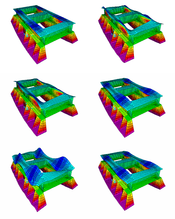
Applications of the Finite Element Method
While renowned for its impact in structural mechanics, the finite element method’s reach extends far beyond. Its potential has been successfully harnessed to address diverse engineering challenges, spanning heat conduction, fluid dynamics, seepage flow, and even the complexities of electric and magnetic fields. This widespread applicability has attracted the attention of mathematicians, who have adopted the method for tackling intricate boundary value problems and beyond.
The underlying foundation of this versatility lies in the ability to numerically solve both ordinary and partial differential equations. By recognizing the underlying similarities between seemingly disparate engineering problems, the finite element method emerges as a unifying tool capable of unlocking solutions across a vast spectrum of disciplines.
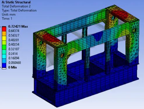
Steps in Finite Element Analysis for Structures
The complex nature of real-world materials, such as solids, liquids, and gases, necessitates their representation in the finite element method as a collection of smaller subdivisions called finite elements. These interconnected elements share specified points of contact known as nodes or nodal points, typically located on their boundaries.
Since the precise variation of a field variable (e.g., displacement, stress, temperature, pressure, or velocity) within the continuum remains unknown, the method assumes that its behavior within each element can be approximated by a simpler function. These approximating functions, also known as interpolation models, are defined based on the nodal values of the field variable.
By formulating field equations (such as equilibrium equations) for the entire continuum, we introduce new unknowns – the nodal values of the field variable. Solving these equations, typically expressed as matrix equations, yields the desired nodal values. With these values in hand, the approximating functions establish the field variable throughout the assemblage of elements. This systematic approach defines the core steps involved in applying the finite element method to diverse problems.
Specifically, considering static structural problems as an example, the step-by-step procedure are as follows:
Step 1: Discretization
The initial stage involves dividing the structure or solution domain into smaller sub-regions called elements. This forms the model representing the actual structure. Careful consideration goes into determining the number, type, size, and arrangement of these elements to ensure an accurate representation.
Step 2: Selecting the Right Displacement Model
Since the exact displacement response of a complex structure under specific loads is unknown, we rely on interpolation models to approximate this behaviour within each element. These models, typically implemented as polynomials, need to be computationally efficient while adhering to convergence requirements essential for accurate solutions.
Step 3: Building the Stiffness Matrices and Load Vectors
Leveraging the chosen displacement model, we derive the stiffness matrix [Ke] and load vector [Pe] for each element. This can be achieved either through equilibrium conditions or a suitable variational principle. The stiffness matrix captures the element’s resistance to deformations, while the load vector represents the external forces acting on it.
Step 4: Assemblage of element equations to obtain the overall equilibrium equations
Since the structure is composed of several finite elements, the individual element stiffness matrices and load vectors are to be assembled in a suitable manner and the overall equilibrium equations have to be formulated as;
[K][Φ] = [P]
where [K] is the assembled stiffness matrix, [Φ] is the vector of nodal displacements, and [P] is the vector of nodal forces for the complete structure.
Step 5: Solution for the unknown nodal displacements
To ensure our model aligns with the real-world structure’s constraints, we incorporate boundary conditions into the overall equilibrium equations. These conditions represent fixed points, support conditions, applied forces, or other restrictions on the structure’s behavior. With these adjustments, the equilibrium equations take the form:
[K]Φ = P
For linear problems, this system of equations can be readily solved using efficient numerical methods, revealing the unknown nodal displacements throughout the structure. However, for nonlinear problems, the complexities introduced by material behavior or large deformations necessitate an iterative approach. Each step in this sequence involves updating the stiffness matrix and/or load vector based on the current solution estimate until convergence is achieved.
Step 6: Computation of element strains and stresses
From the known nodal displacements (Φ), if required, the element strains and stresses can be computed by using the necessary equations of solid or structural mechanics.
Code Snippet for FEA of Trusses on Python
To bridge the gap between theory and practice, let’s explore fundamental FEA concepts through code snippets in a chosen programming language (e.g., Python). We’ll demonstrate element stiffness matrix formulation for simple elements like trusses, followed by global system assembly and solution using basic numerical libraries.
- Import necessary libraries
import numpy as np

# If needed for solving linear systems:
import scipy.linalg as la
2. Define truss element properties:
def element_stiffness_matrix(E, A, L):
    """Calculates the 2x2 stiffness matrix for a truss element."""
    ke = E * A / L * np.array([[1, -1], [-1, 1]])
    return ke

def element_load_vector(q, L):
    """Calculates the 2x1 load vector for a truss element."""
    fe = q * L / 2 * np.array([[1], [1]])
    return fe
3. Assemble global stiffness matrix and load vector
def assemble_global_system(elements, nodes):
    """Assembles the global stiffness matrix and load vector."""
    K = np.zeros((nodes * 2, nodes * 2))
    P = np.zeros((nodes * 2, 1))
    for element in elements:
        node1, node2, E, A, L, q = element
        ke = element_stiffness_matrix(E, A, L)
        fe = element_load_vector(q, L)
        d = 2 * (node1 - 1)  # Global degree of freedom indices
        K[d:d+2, d:d+2] += ke
        P[d:d+2] += fe
    return K, P
4. Apply boundary conditions:
def apply_boundary_conditions(K, P, fixed_nodes, fixed_values):
    """Applies boundary conditions to the global system."""
    for node, value in zip(fixed_nodes, fixed_values):
        d = 2 * (node - 1)
        K[d:d+2, :] = 0
        K[:, d:d+2] = 0
        K[d, d] = 1
        P[d] = value
5. Solve for nodal displacements
def solve_displacements(K, P):
    """Solves the system of equations for nodal displacements."""
    U = la.solve(K, P)
    return U
6. Calculate element stresses and reactions:
def calculate_stresses(elements, U):
    # ... (Implementation for stress calculation based on element type)

def calculate_reactions(K, U, fixed_nodes):
    # ... (Implementation for reaction force calculation)
Conclusion
This article has provided a foundational understanding of FEA, its theoretical principles, and practical implementation through code snippets. By delving deeper into specific element types, advanced material models, and non-linear analysis, beginners can progressively build their FEA skillset and tackle increasingly complex engineering problems.

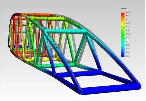


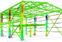


Treat particular design specific:
Roof trusses for an auditorium 34.04m wide and 54m length.
There are stepped galleries on first floor Each gallery step is 5.5m wide floor permitting sitting and passage. Structured rare column 600mm diameter middle stepped floor 5.2m wide with a square column spaced at y-axis 5m from circular column rear column and 4.5 m to inner circular column. x-axis spacing 10m each centre to centre. This arrangement repeats on the opposite side forming a void between them. roof beams roud the four sides of the structure. Roof beam built at a stunning height of 5.5m from the first floor external column level.
Design a suitable roof truss to carry roof sheets on Z purlins.
Thank you!